Skew-T and hodograph

The 18 UTC special sounding from Birmingham, Alabama on 27 April 2011, launched a few hours before the day's long-track tornadoes. The surface parcel is lifted dry to its condensation level and moist above it, with its CAPE and CIN shaded. The hodograph is coloured by height above ground.

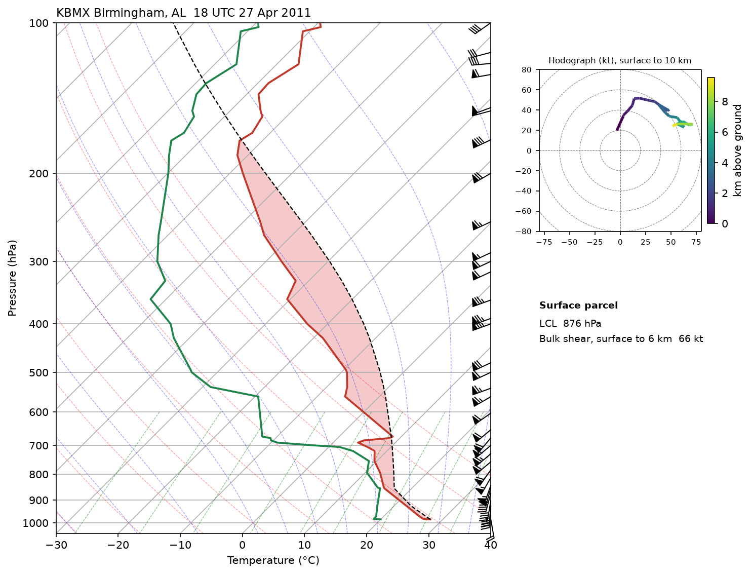
Data: Iowa Environmental Mesonet radiosonde archive, saved in docs/examples/data/raob_KBMX_2011042718.csv.

docs/examples/sounding.py

"""The 18 UTC special sounding from Birmingham, Alabama on 27 April 2011,
launched hours before the day's long-track tornadoes: the surface parcel's
CAPE and CIN on a Skew-T, and the wind profile on a hodograph coloured by
height. Data from the Iowa Environmental Mesonet's radiosonde archive."""
import os

import numpy as np

import fastplot.pyplot as plt
from fastplot.skewt import Hodograph, SkewT, dry_lapse, moist_lapse

HERE = os.path.dirname(os.path.abspath(__file__))
raob = np.genfromtxt(os.path.join(HERE, 'data', 'raob_KBMX_2011042718.csv'), delimiter=',',
                     names=True)
thermo = np.isfinite(raob['temp_c']) & np.isfinite(raob['dewp_c'])
p, T, Td = raob['pres_hpa'][thermo], raob['temp_c'][thermo], raob['dewp_c'][thermo]
windy = np.isfinite(raob['sknt_kt']) & np.isfinite(raob['drct_deg']) & (raob['pres_hpa'] >= 100)
pw, zw = raob['pres_hpa'][windy], raob['hght_m'][windy] - raob['hght_m'][thermo][0]
u = -raob['sknt_kt'][windy] * np.sin(np.radians(raob['drct_deg'][windy]))
v = -raob['sknt_kt'][windy] * np.cos(np.radians(raob['drct_deg'][windy]))

# The surface parcel: dry to its lifting condensation level (Bolton 1980), moist above.
t0, td0 = T[0] + 273.15, Td[0] + 273.15
t_lcl = 1.0 / (1.0 / (td0 - 56.0) + np.log(t0 / td0) / 800.0) + 56.0
p_lcl = p[0] * (t_lcl / t0) ** (1 / 0.2857)
parcel = np.where(p >= p_lcl, dry_lapse(p, t0, p[0]), moist_lapse(p, t_lcl, p_lcl)) - 273.15
u6, v6 = np.interp(6000, zw, u), np.interp(6000, zw, v)

fig = plt.figure(figsize=(10, 8), dpi=150)
skew = SkewT(fig, rotation=45, rect=(0.07, 0.08, 0.58, 0.84))
skew.plot_dry_adiabats(linewidth=0.6, alpha=0.4)
skew.plot_moist_adiabats(linewidth=0.6, alpha=0.4)
skew.plot_mixing_lines(linewidth=0.6, alpha=0.5)
skew.shade_cape(p, T, parcel, alpha=0.25)
skew.shade_cin(p, T, parcel, Td, alpha=0.25)
skew.plot(p, T, color='#c0392b', linewidth=1.8)
skew.plot(p, Td, color='#1e8449', linewidth=1.8)
skew.plot(p, parcel, color='black', linewidth=1.1, linestyle='--')
step = max(1, pw.size // 25)
skew.plot_barbs(pw[::step], u[::step], v[::step], length=6)
skew.ax.set_xlim(-30, 40)
skew.ax.set_xlabel('Temperature (°C)')
skew.ax.set_ylabel('Pressure (hPa)')
skew.ax.set_title('KBMX Birmingham, AL  18 UTC 27 Apr 2011', loc='left', fontsize=11)

hodo_ax = fig.add_axes((0.71, 0.56, 0.26, 0.3))
hodo = Hodograph(hodo_ax, component_range=80)
hodo.add_grid(increment=20, linewidth=0.5)
low = zw <= 10000
line = hodo.plot_colormapped(u[low], v[low], zw[low] / 1000, cmap='viridis', linewidth=2.5)
fig.colorbar(line, ax=hodo_ax, shrink=0.8, pad=0.03, label='km above ground')
hodo_ax.set_title('Hodograph (kt), surface to 10 km', fontsize=8)
hodo_ax.tick_params(labelsize=7)

fig.text(0.71, 0.45, 'Surface parcel', fontsize=9, fontweight='bold')
fig.text(0.71, 0.42, 'LCL  %.0f hPa' % p_lcl, fontsize=9)
fig.text(0.71, 0.395, 'Bulk shear, surface to 6 km  %.0f kt' % np.hypot(u6 - u[0], v6 - v[0]),
         fontsize=9)

fig.savefig(os.path.join(HERE, '..', 'images', 'sounding.png'), bbox_inches='tight')