Quasi-geostrophic forcing and model ascent
Q-vectors and the forcing term of the QG omega equation, -2 div Q, computed from the GFS 700 hPa height and temperature with the geostrophic wind, next to the model's own vertical motion at the same level. Q-vectors converge where the large-scale balanced flow forces ascent. Where the two panels agree, as ahead of the trough over the western Atlantic, the model's ascent is that balanced response; where they differ, convection, terrain or the tropics are at work.
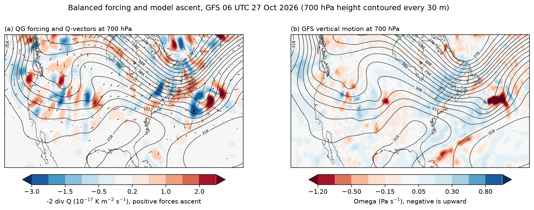
Data: GFS 0.5°, 00 UTC 27 October 2026, six-hour forecast, read with fastgrib from NOAA's archive on AWS by byte range. The loading and finite-difference code is shared with the other diagnostics in docs/examples/gfs3d.py.
docs/examples/qg_forcing.py
"""Quasi-geostrophic forcing for vertical motion against the model's own
vertical motion, at 700 hPa over North America and the western Atlantic.

(a) Q-vectors (arrows) and the forcing term of the QG omega equation,
    -2 div Q, computed from the GFS height and temperature at 700 hPa:

        Q = -(R/p) ( dVg/dx . grad T ,  dVg/dy . grad T ),

    with the geostrophic wind Vg = (g/f) k x grad Z. Q converges where
    balanced dynamics forces ascent (red) and diverges where it forces
    descent (blue). Heights and temperatures are smoothed to synoptic scales
    first, since QG theory describes the large-scale balanced flow.
(b) The GFS's own vertical motion at 700 hPa (omega, Pa s^-1; negative is
    upward). Where the two agree, the model's ascent is the balanced
    response to the large-scale flow; where they differ (convection, terrain,
    the tropics) something QG theory leaves out is at work.
"""
import os

import numpy as np

import fastplot.crs as ccrs
import fastplot.pyplot as plt
import gfs3d

grib = gfs3d.open_gfs()
lat, lon = gfs3d.axes(grib)
z, t, omega = (gfs3d.levels(grib, n, (700,))[0] for n in ('HGT', 'TMP', 'VVEL'))

z, t = gfs3d.smooth(z, 12), gfs3d.smooth(t, 12)
f = gfs3d.coriolis(lat) * np.ones_like(z)
f = np.where(np.abs(lat)[:, None] >= 15, f, np.nan)                   # no balance near the equator
ug, vg = -gfs3d.G / f * gfs3d.ddy(z, lat), gfs3d.G / f * gfs3d.ddx(z, lat, lon)
tx, ty = gfs3d.ddx(t, lat, lon), gfs3d.ddy(t, lat)
rp = 287.04 / 70000.0
q1 = -rp * (gfs3d.ddx(ug, lat, lon) * tx + gfs3d.ddx(vg, lat, lon) * ty)
q2 = -rp * (gfs3d.ddy(ug, lat) * tx + gfs3d.ddy(vg, lat) * ty)
forcing = gfs3d.smooth(-2 * (gfs3d.ddx(q1, lat, lon) + gfs3d.ddy(q2, lat)), 3) * 1e17
omega = gfs3d.smooth(omega, 2)

data = ccrs.PlateCarree()
proj = ccrs.LambertConformal(central_longitude=-85, central_latitude=42)
fig, axes = plt.subplots(1, 2, figsize=(15, 5.0), dpi=150, subplot_kw={'projection': proj})

for ax in axes:
    ax.set_extent([-125, -45, 25, 60], crs=data)
    ax.coastlines(linewidth=0.5, color='#333333')
    heights = ax.contour(lon, lat, z / 10, levels=np.arange(270, 330, 3), colors='black',
                         linewidths=0.6, transform=data)
    ax.clabel(heights, levels=heights.levels[::2], fmt='%d', fontsize=6)

ax = axes[0]
filled = ax.contourf(lon, lat, forcing, levels=[-3, -2, -1.5, -1, -0.5, -0.2, 0.2, 0.5, 1, 1.5, 2, 3],
                     cmap='RdBu_r', extend='both', transform=data)
step = 7
qx, qy = np.meshgrid(lon[::step], lat[::step])
sub = (slice(None, None, step), slice(None, None, step))
ax.quiver(qx, qy, q1[sub], q2[sub], scale=3e-11, width=0.0016, color='#333333',
          transform=data)
fig.colorbar(filled, ax=ax, orientation='horizontal', pad=0.04, shrink=0.85,
             label='-2 div Q (10$^{-17}$ K m$^{-2}$ s$^{-1}$), positive forces ascent')
ax.set_title('(a) QG forcing and Q-vectors at 700 hPa', loc='left', fontsize=10)

ax = axes[1]
filled = ax.contourf(lon, lat, omega, levels=[-1.2, -0.8, -0.5, -0.3, -0.15, -0.05, 0.05, 0.15,
                                              0.3, 0.5, 0.8, 1.2],
                     cmap='RdBu', extend='both', transform=data)
fig.colorbar(filled, ax=ax, orientation='horizontal', pad=0.04, shrink=0.85,
             label='Omega (Pa s$^{-1}$), negative is upward')
ax.set_title('(b) GFS vertical motion at 700 hPa', loc='left', fontsize=10)

fig.suptitle('Balanced forcing and model ascent, GFS 06 UTC 27 Oct 2026 (700 hPa height '
             'contoured every 30 m)', fontsize=12)
fig.savefig(os.path.join(os.path.dirname(os.path.abspath(__file__)), '..', 'images',
                         'qg_forcing.png'), bbox_inches='tight')
docs/examples/gfs3d.py, shared by the diagnostics
"""Shared by the diagnostic examples: GFS fields on pressure levels, read with
fastgrib, and the finite differences on a sphere the diagnostics are built
from.

The fields come from the GFS 0.5° run of 00 UTC 27 October 2026, six-hour
forecast, in NOAA's archive on AWS. fastgrib reads the file's index and
fetches only the records asked for. Set GFS_FILE_0P50 to read a local copy.
"""
import os

import numpy as np

import fastgrib

URL = 'https://noaa-gfs-bdp-pds.s3.amazonaws.com/gfs.20261027/00/atmos/gfs.t00z.pgrb2.0p50.f006'
LEVELS = (1000, 975, 950, 925, 900, 850, 800, 750, 700, 650, 600, 550, 500, 450, 400, 350,
          300, 250, 200, 150, 100, 70, 50)                     # hPa, bottom to top

R_EARTH = 6.371e6          # m
G = 9.80665                # m s-2
OMEGA = 7.2921e-5          # s-1
KAPPA = 0.2857             # R_d / c_p


def open_gfs():
    return fastgrib.open(os.environ.get('GFS_FILE_0P50', URL))


def levels(grib, name, levels=LEVELS):
    """One variable on the given pressure levels, as (level, lat, lon), bottom
    to top. All records are fetched in one call."""
    recs = grib.select(name=name, level_kind='isobaricInhPa',
                       level_value=lambda v: v in set(levels))
    recs = sorted(recs, key=lambda r: -r.level_value)
    if [r.level_value for r in recs] != list(levels):
        raise ValueError('%s: levels %s' % (name, [r.level_value for r in recs]))
    data = grib.read(recs).astype(np.float64)
    return data[None] if data.ndim == 2 else data          # one level: still (1, lat, lon)


def axes(grib):
    """The grid's 1-D latitudes (south to north) and longitudes (east from 0)."""
    lat, lon = grib.latlon()
    return lat[:, 0].astype(np.float64), lon[0].astype(np.float64)


def ddx(f, lat, lon):
    """d/dx on the sphere along the last axis, periodic in longitude."""
    dlam = np.radians(lon[1] - lon[0])
    dfdl = (np.roll(f, -1, axis=-1) - np.roll(f, 1, axis=-1)) / (2 * dlam)
    coslat = np.maximum(np.cos(np.radians(lat)), 1e-6)[:, None]
    return dfdl / (R_EARTH * coslat)


def ddy(f, lat):
    """d/dy on the sphere along the second-last axis."""
    return np.gradient(f, np.radians(lat), axis=-2) / R_EARTH


def ddp(f, p_hpa):
    """d/dp along the first axis, p in Pa (levels need not be evenly spaced)."""
    return np.gradient(f, np.asarray(p_hpa, np.float64) * 100.0, axis=0)


def coriolis(lat):
    return 2 * OMEGA * np.sin(np.radians(lat))[:, None]


def vorticity(u, v, lat, lon):
    """Relative vorticity, with the curvature term of a spherical grid."""
    tan = np.tan(np.radians(lat))[:, None]
    return ddx(v, lat, lon) - ddy(u, lat) + u * tan / R_EARTH


def theta(t, p_hpa):
    """Potential temperature of temperature t (K) at pressure p (hPa, along axis 0
    or a scalar)."""
    p = np.asarray(p_hpa, np.float64)
    if p.ndim:
        p = p[:, None, None]
    return t * (1000.0 / p) ** KAPPA


def smooth(f, passes=1):
    """A 9-point smoother on the last two axes, periodic in longitude."""
    for _ in range(passes):
        g = np.concatenate([f[..., :1, :], f, f[..., -1:, :]], axis=-2)
        g = np.concatenate([g[..., -1:], g, g[..., :1]], axis=-1)
        sides = g[..., 2:, 1:-1] + g[..., :-2, 1:-1] + g[..., 1:-1, 2:] + g[..., 1:-1, :-2]
        corners = g[..., 2:, 2:] + g[..., 2:, :-2] + g[..., :-2, 2:] + g[..., :-2, :-2]
        f = (4 * g[..., 1:-1, 1:-1] + 2 * sides + corners) / 16
    return f


def bilinear(f, lat, lon, plat, plon):
    """f (..., lat, lon) at points (plat, plon) by bilinear interpolation."""
    j = np.interp(plat, lat, np.arange(lat.size))
    i = ((np.asarray(plon) - lon[0]) % 360.0) / (lon[1] - lon[0])
    j0 = np.clip(np.floor(j).astype(int), 0, lat.size - 2)
    i0 = np.floor(i).astype(int) % lon.size
    i1 = (i0 + 1) % lon.size
    wj, wi = j - j0, i - np.floor(i)
    return ((1 - wj) * ((1 - wi) * f[..., j0, i0] + wi * f[..., j0, i1])
            + wj * ((1 - wi) * f[..., j0 + 1, i0] + wi * f[..., j0 + 1, i1]))