Hurricane vortex structure

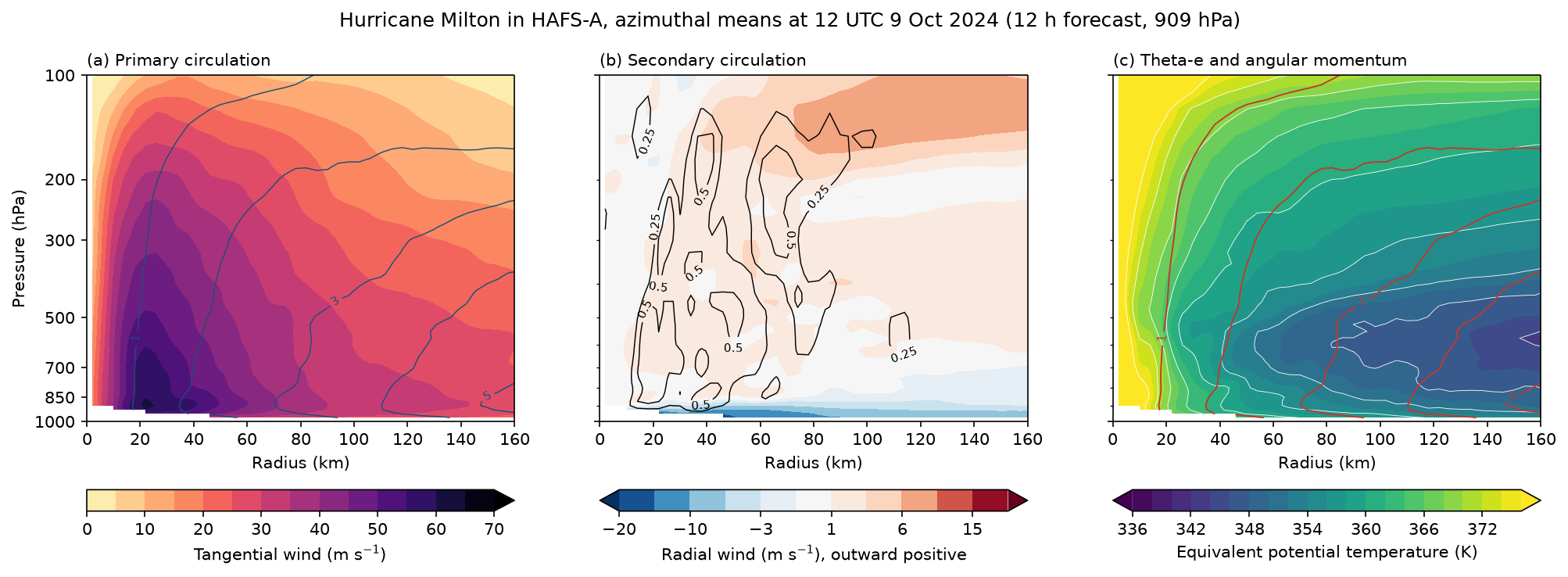
Azimuthal means around Hurricane Milton 12 hours into the HAFS-A forecast from 00 UTC 9 October 2024, in storm-relative coordinates: the primary circulation (tangential wind) with surfaces of absolute angular momentum, the secondary circulation (inflow, outflow and the eyewall updraught), and equivalent potential temperature from Bolton (1980) against the same angular momentum surfaces. In Emanuel's theory of the mature hurricane the eyewall is neutral to slantwise convection, so theta-e surfaces lie along M surfaces there; between 20 and 60 km from the centre they do.

Data: HAFS-A storm nest from NOAA's HAFS archive on AWS (noaa-nws-hafs-pds), about 180 records fetched by byte range.

docs/examples/hafs_milton.py

"""The azimuthal-mean structure of Hurricane Milton in HAFS-A, 12 hours into the
forecast from 00 UTC 9 October 2024, a day before landfall in Florida. All
three panels are averages around the storm centre against radius and
pressure, in storm-relative coordinates.

(a) Primary circulation: tangential wind, with surfaces of absolute angular
    momentum M = r v + f r^2 / 2 (10^6 m^2 s^-1).
(b) Secondary circulation: radial wind, inflow in the lowest 100 hPa and
    outflow near 150 hPa, with the eyewall updraught (vertical velocity
    contoured in m s^-1) joining them.
(c) Slantwise neutrality: equivalent potential temperature (Bolton 1980),
    with the same angular momentum surfaces. Emanuel's theory of the mature
    hurricane has the eyewall neutral to slantwise moist convection, so that
    surfaces of theta-e lie along surfaces of M. In the eyewall, 20-60 km
    from the centre, they do.

The storm centre is the sea-level pressure minimum within 50 km of HAFS-A's
own track position, and the storm motion comes from that track's positions
at 9 and 15 hours. Fields come from the 2 km storm nest in NOAA's HAFS
archive on AWS, one byte range per record.
"""
import os

import numpy as np

import fastgrib
import fastplot.pyplot as plt

BASE = 'https://noaa-nws-hafs-pds.s3.amazonaws.com/hfsa/20241009/00/14l.2024100900.hfsa.'
R_EARTH = 6.371e6
LEVELS = list(range(1000, 99, -25))                                       # hPa

atm = fastgrib.open(BASE + 'storm.atm.f012.grb2')
lat, lon = atm.latlon()
lat, lon = lat[:, 0].astype(float), lon[0].astype(float) - 360.0


def column(name):
    recs = atm.select(name=name, level_kind='isobaricInhPa',
                      level_value=lambda v: v in set(LEVELS))
    recs = sorted(recs, key=lambda r: -r.level_value)
    return atm.read(recs).astype(float)


# The centre: the pressure minimum near HAFS-A's track position at 12 h.
track = {9: (24.4, -85.6), 12: (24.9, -85.2), 15: (25.4, -84.8)}
mslp = atm.read('PRMSL:mean sea level').astype(float)
near = (np.abs(lat[:, None] - track[12][0]) < 0.45) & (np.abs(lon[None] - track[12][1]) < 0.5)
j, i = np.unravel_index(np.argmin(np.where(near, mslp, np.inf)), mslp.shape)
clat, clon = lat[j], lon[i]
coslat = np.cos(np.radians(clat))
x = R_EARTH * coslat * np.radians(lon[None] - clon) / 1000.0              # km east
y = R_EARTH * np.radians(lat[:, None] - clat) / 1000.0                    # km north
r = np.hypot(x, y)
cx = R_EARTH * coslat * np.radians(track[15][1] - track[9][1]) / (6 * 3600)
cy = R_EARTH * np.radians(track[15][0] - track[9][0]) / (6 * 3600)

u, v = column('UGRD') - cx, column('VGRD') - cy
t, w, q = column('TMP'), column('DZDT'), column('SPFH')
psfc = atm.read('PRES:surface').astype(float) / 100.0
p3 = np.array(LEVELS, float)[:, None, None]

# Equivalent potential temperature, Bolton (1980) eq. 43, from mixing ratio
# and the temperature at the lifting condensation level (eq. 21).
mix = q / (1 - q)                                                          # kg kg-1
e = np.maximum(p3 * mix / (0.622 + mix), 1e-6)                             # hPa
t_lcl = 2840.0 / (3.5 * np.log(t) - np.log(e) - 4.805) + 55.0
theta_e = (t * (1000.0 / p3) ** (0.2854 * (1 - 0.28 * mix))
           * np.exp((3.376 / t_lcl - 0.00254) * 1000 * mix * (1 + 0.81 * mix)))

with np.errstate(invalid='ignore', divide='ignore'):
    vt = (-u * y + v * x) / r                                             # cyclonic positive
    vr = (u * x + v * y) / r                                              # outward positive
edges = np.arange(0, 302, 4.0)
ring = np.digitize(r, edges) - 1
inside = (ring >= 0) & (ring < edges.size - 1)
radius = 0.5 * (edges[1:] + edges[:-1])


def azimuthal_mean(f):
    """Mean of f (level, lat, lon) in each ring, leaving out points below ground."""
    out = np.full((len(LEVELS), radius.size), np.nan)
    for k, p in enumerate(LEVELS):
        ok = inside & (psfc > p) & np.isfinite(f[k])
        total = np.bincount(ring[ok], f[k][ok], minlength=radius.size)
        count = np.bincount(ring[ok], minlength=radius.size)
        with np.errstate(invalid='ignore', divide='ignore'):
            out[k] = total / count
    return out


vt_m, vr_m, w_m, the_m = (azimuthal_mean(a) for a in (vt, vr, w, theta_e))
f = 2 * 7.2921e-5 * np.sin(np.radians(clat))
ang_mom = (radius * 1000 * vt_m + 0.5 * f * (radius * 1000) ** 2) / 1e6  # 10^6 m^2 s^-1
p = np.array(LEVELS, float)
m_levels = np.arange(1, 13, 1)

fig, axes = plt.subplots(1, 3, figsize=(16, 5.4), dpi=150, sharey=True)
ax1, ax2, ax3 = axes

filled = ax1.contourf(radius, p, vt_m, levels=np.arange(0, 71, 5), cmap='magma_r',
                      extend='max')
mom = ax1.contour(radius, p, ang_mom, levels=m_levels, colors='#1b4f72', linewidths=0.7)
ax1.clabel(mom, levels=mom.levels[::2], fmt='%d', fontsize=7)
fig.colorbar(filled, ax=ax1, orientation='horizontal', pad=0.14,
             label='Tangential wind (m s$^{-1}$)')
ax1.set_title('(a) Primary circulation', loc='left', fontsize=10)

flow = ax2.contourf(radius, p, vr_m, levels=[-20, -15, -10, -6, -3, -1, 1, 3, 6, 10, 15, 20],
                    cmap='RdBu_r', extend='both')
updraught = ax2.contour(radius, p, w_m, levels=[0.25, 0.5, 1, 1.5, 2], colors='black',
                        linewidths=0.7)
ax2.clabel(updraught, fmt='%g', fontsize=7)
fig.colorbar(flow, ax=ax2, orientation='horizontal', pad=0.14,
             label='Radial wind (m s$^{-1}$), outward positive')
ax2.set_title('(b) Secondary circulation', loc='left', fontsize=10)

moist = ax3.contourf(radius, p, the_m, levels=np.arange(336, 377, 2), cmap='viridis',
                     extend='both')
ax3.contour(radius, p, the_m, levels=np.arange(336, 377, 4), colors='white',
            linewidths=0.4)
mom = ax3.contour(radius, p, ang_mom, levels=m_levels, colors='#c0392b', linewidths=0.9)
ax3.clabel(mom, levels=mom.levels[::2], fmt='%d', fontsize=7)
fig.colorbar(moist, ax=ax3, orientation='horizontal', pad=0.14,
             label='Equivalent potential temperature (K)')
ax3.set_title('(c) Theta-e and angular momentum', loc='left', fontsize=10)

ax1.set_yscale('log')
ax1.set_ylim(1000, 100)
ax1.set_yticks([1000, 850, 700, 500, 300, 200, 100],
               ['1000', '850', '700', '500', '300', '200', '100'])
ax1.minorticks_off()
ax1.set_ylabel('Pressure (hPa)')
for ax in axes:
    ax.set_xlim(0, 160)
    ax.set_xlabel('Radius (km)')

fig.suptitle('Hurricane Milton in HAFS-A, azimuthal means at 12 UTC 9 Oct 2024 '
             '(12 h forecast, %.0f hPa)' % (mslp[j, i] / 100), fontsize=12)

fig.savefig(os.path.join(os.path.dirname(os.path.abspath(__file__)), '..', 'images',
                         'hafs_milton.png'), bbox_inches='tight')