Ensemble sensitivity

The 31 GEFS members disagree most at day 5 near Kamchatka. Correlating the members' day-5 500 hPa height in a box there with their day-2 heights everywhere (Ancell and Hakim 2007) shows where differences at day 2 grow into that uncertainty: the trough upstream and the ridge to its south. Black contours mark correlations significant at 95%.

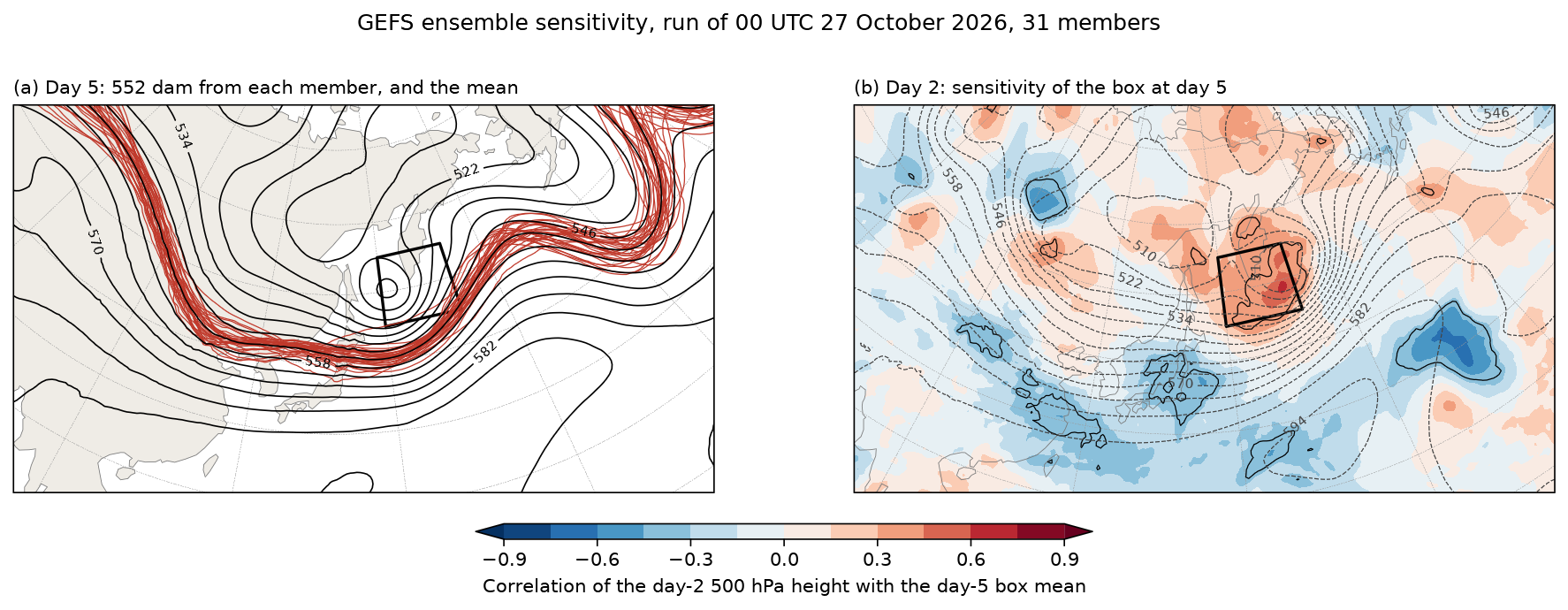
Data: GEFS 0.5°, 00 UTC 27 October 2026, 48- and 120-hour forecasts, 62 fields from separate member files.

docs/examples/ensemble_sensitivity.py

"""Ensemble sensitivity: which part of the day-2 forecast decides an uncertain
day-5 forecast, from the 31 members of the GEFS run of 00 UTC 27 October
2026.

(a) Day 5. The 552 dam contour of 500 hPa height from every member, over the
    ensemble mean, near Kamchatka, where the members disagree most (a spread
    of 88 m). The box is the response: J, the mean 500 hPa height inside it.
(b) Day 2. The correlation, across the 31 members, between J and the 500 hPa
    height at each point at day 2 (Ancell and Hakim 2007), over the ensemble
    mean. Where it is strong, members that put that part of the flow higher
    (red) or lower (blue) at day 2 also have the box higher at day 5:
    errors there grow into the day-5 uncertainty. Black contours mark
    |r| = 0.36, the 95% significance level for 31 members.

The 62 fields come from separate member files in NOAA's GEFS archive on AWS;
fastgrib fetches one field from each.
"""
import os
from concurrent.futures import ThreadPoolExecutor

import numpy as np

import fastgrib
import fastplot.crs as ccrs
import fastplot.feature as cfeature
import fastplot.pyplot as plt

URL = ('https://noaa-gefs-pds.s3.amazonaws.com/gefs.20261027/00/atmos/pgrb2ap5/'
       '{}.t00z.pgrb2a.0p50.f{:03d}')
members = ['gec00'] + ['gep%02d' % k for k in range(1, 31)]
BOX = (45.0, 55.0, 150.0, 166.0)                       # lat, lat, lon east, lon east


def height(job):
    member, hour = job
    return fastgrib.open(URL.format(member, hour)).read('HGT:500 mb').astype(np.float64) / 10


with ThreadPoolExecutor(8) as pool:
    z48 = np.array(list(pool.map(height, [(m, 48) for m in members])))
    z120 = np.array(list(pool.map(height, [(m, 120) for m in members])))
lat = np.arange(-90, 90.5, 0.5)
lon = np.arange(0, 360, 0.5)

rows = (lat >= BOX[0]) & (lat <= BOX[1])
cols = (lon >= BOX[2]) & (lon <= BOX[3])
weight = np.cos(np.radians(lat[rows]))[:, None]
response = (z120[:, rows][:, :, cols] * weight).sum(axis=(1, 2)) / (weight.sum() * cols.sum())

anom = z48 - z48.mean(axis=0)
ja = response - response.mean()
corr = (anom * ja[:, None, None]).sum(axis=0) / np.sqrt(
    (anom ** 2).sum(axis=0) * (ja ** 2).sum())

data = ccrs.PlateCarree()
proj = ccrs.LambertConformal(central_longitude=140, central_latitude=45,
                             standard_parallels=(35, 55))
fig, axes = plt.subplots(1, 2, figsize=(15, 5.1), dpi=150, subplot_kw={'projection': proj})
for ax in axes:
    ax.set_extent([90, 200, 22, 68], crs=data)
    ax.add_feature(cfeature.LAND, facecolor='#efece6')
    ax.coastlines(linewidth=0.4, color='#777777')
    ax.gridlines(linewidth=0.25, color='#999999', linestyle='--')
    ax.plot([BOX[2], BOX[3], BOX[3], BOX[2], BOX[2]], [BOX[0], BOX[0], BOX[1], BOX[1], BOX[0]],
            color='black', linewidth=1.6, transform=data)

ax = axes[0]
for member in z120:
    ax.contour(lon, lat, member, levels=[552], colors='#c0392b', linewidths=0.6,
               transform=data)
mean = ax.contour(lon, lat, z120.mean(axis=0), levels=np.arange(510, 600, 6), colors='black',
                  linewidths=0.8, transform=data)
ax.clabel(mean, levels=mean.levels[::2], fmt='%d', fontsize=7)
ax.set_title('(a) Day 5: 552 dam from each member, and the mean', loc='left', fontsize=10)

ax = axes[1]
filled = ax.contourf(lon, lat, corr, levels=np.arange(-0.9, 0.91, 0.15), cmap='RdBu_r',
                     extend='both', transform=data)
ax.contour(lon, lat, np.abs(corr), levels=[0.36], colors='black', linewidths=0.6,
           transform=data)
mean = ax.contour(lon, lat, z48.mean(axis=0), levels=np.arange(510, 600, 6), colors='#444444',
                  linewidths=0.6, linestyles='--', transform=data)
ax.clabel(mean, levels=mean.levels[::2], fmt='%d', fontsize=7)
fig.colorbar(filled, ax=axes, orientation='horizontal', shrink=0.4, pad=0.06, aspect=40,
             label='Correlation of the day-2 500 hPa height with the day-5 box mean')
ax.set_title('(b) Day 2: sensitivity of the box at day 5', loc='left', fontsize=10)

fig.suptitle('GEFS ensemble sensitivity, run of 00 UTC 27 October 2026, 31 members',
             fontsize=12)
fig.savefig(os.path.join(os.path.dirname(os.path.abspath(__file__)), '..', 'images',
                         'ensemble_sensitivity.png'), bbox_inches='tight')